Implementing the Word2Vec model in JAX
Understanding the nuts and bolts of Word2Vec by fully implementing it in JAX.
⚠️🚧 This post is under construction ⚠️🚧
This tutorial provides a complete step-by-step implementation of the Word2Vec model developed by Mikolov et al. (2013) using JAX.
0. Setup
import sys
import pandas as pd
import numpy as np
from scipy import spatial

import jax
import jax.numpy as jnp
from jax import grad, jit, vmap, value_and_grad
from jax import value_and_grad
import jax.nn as nn
from jax.random import PRNGKey as Key
from collections import Counter
import time
from jax.experimental import optimizers
import nltk
import string
import re
import math
import pickle
import random

import matplotlib
import matplotlib.pyplot as plt
from sklearn.decomposition import PCA
import seaborn as sns
from scipy import spatial
from annoy import AnnoyIndex
from IPython import display

import preprocessing_class as pc
1. Data Generation: The Skipgram model
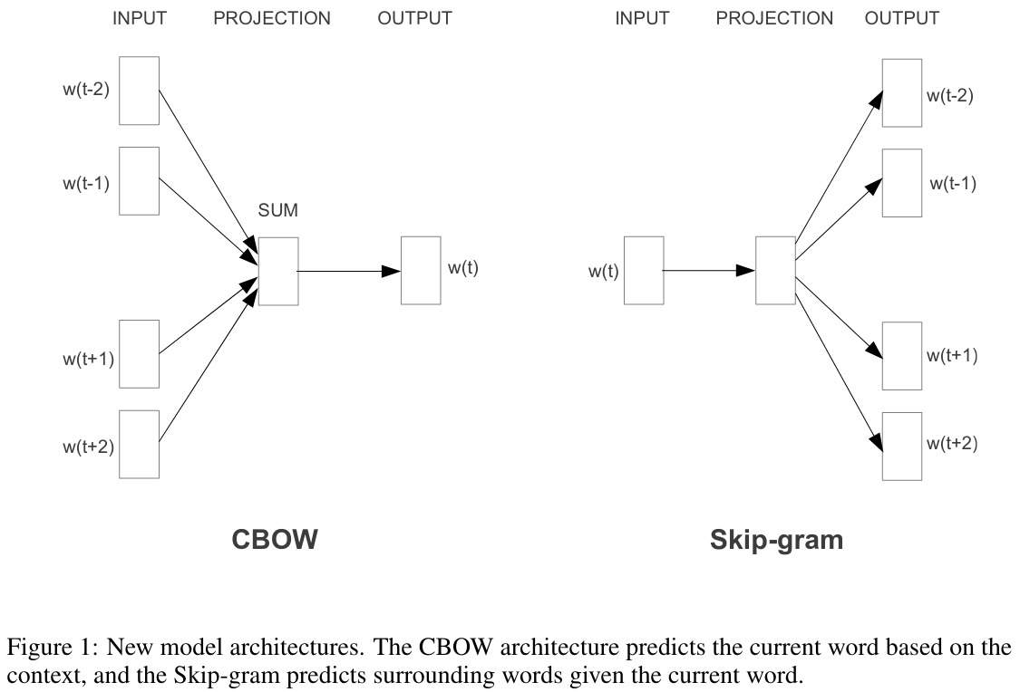
Word2Vec relies on a very simple, but powerful, intuition about text data; the order of the words contains valuable information. Instead of transforming all text into a bag-of-words representation, Word2Vec uses the order of the words to define a prediction task. Concretely, this task can be formulated in two different ways:
-
Continous Bag of Words (CBOW): Predict a word given the words in it’s context. We want to model
\[Pr(w_t | w_{t-2}, w_{t-1}, w_{t+1}, w_{t+2})\] -
Skip-gram: Model the context given a center word. We want to model
\[Pr(w_{t-2}, w_{t-1}, w_{t+1}, w_{t+2} | w_t)\]
The figure below (Mikolov et al. (2013)) clearly shows these 2 different prediction tasks. In this tutorial we will focus on the skip-gram model.
display.Image("images/cbow_skipgram.png", width=1200, height=800)
def skipgram_examples(corpus, vocab_dict, window=2):
    """ Function to identify center and context words in the provided corpus.
        Examples are only generated for words that are in a position in which
        sufficient context words are available (window*2).

    Args:
        corpus (list): containing each document of the corpus represented
        as a list of tokens

        vocab_dict (dict): mapping words to their index representation

        window (int): window*2 will be the total number of words considered
        as context; (window) words before and (window) words after the
        selected center word

    Returns:
        jax array of indexes representing each center word in the corpus
        jax array of jax arrays representing the indexes of context words
    """

    # lists to store the results
    centers = []
    contexts = []

    # iterate over al documents in the corpus
    for doc in corpus:

        center = window
        while center < (len(doc)-window):
            # save the current center word
            centers.append(vocab_dict[doc[center]])
            # create a list to store the context of the current center
            context_words = []
            # search for context
            for i in range(0, (window*2)+1):
                if (center-window+i) != center:
                    context_words.append(vocab_dict[doc[center-window+i]])

            # append all the context words identified
            contexts.append(context_words)
            # update center
            center += 1

    return jnp.array(centers), jnp.array(contexts)
1.1. Load data and preprocess text
We will now load some real data in order to understand the data structure that we are generating for the skip-gram model. We see that our data consists of paragraphs from the Inflation Reports produced by the Bank of England. The data starts on 1998 and ends in 2015. Reports are produced fours times a year in the months of February, May, August and November.
data = pd.read_csv("ir_data_final.txt", sep="\t")
data["year"] = pd.to_datetime(data['ir_date'], format='%Y%m')
data['yearmonth'] = data["year"].dt.strftime("%Y%m")
print(data.shape)
data.head(10)
(15023, 9)
| ir_date | paragraph | section | sub_section | sub_sub_section | sub_sub_sub_section | sub_sub_sub_sub_section | year | yearmonth | |
|---|---|---|---|---|---|---|---|---|---|
| 0 | 199802 | It is almost six years since output reached it... | 0.0 | NaN | NaN | NaN | NaN | 1998-02-01 | 199802 |
| 1 | 199802 | Monetary policy is currently being pulled in o... | 0.0 | NaN | NaN | NaN | NaN | 1998-02-01 | 199802 |
| 2 | 199802 | On the other hand, the delayed demand effect o... | 0.0 | NaN | NaN | NaN | NaN | 1998-02-01 | 199802 |
| 3 | 199802 | The scale of the slowdown depends, in part, on... | 0.0 | NaN | NaN | NaN | NaN | 1998-02-01 | 199802 |
| 4 | 199802 | Net trade is weakening, but domestic demand gr... | 0.0 | NaN | NaN | NaN | NaN | 1998-02-01 | 199802 |
| 5 | 199802 | The combination of sharply weakening net trade... | 0.0 | NaN | NaN | NaN | NaN | 1998-02-01 | 199802 |
| 6 | 199802 | The MPC’s probability distribution for the fou... | 0.0 | NaN | NaN | NaN | NaN | 1998-02-01 | 199802 |
| 7 | 199802 | The MPC’s projection of the twelve-month RPIX ... | 0.0 | NaN | NaN | NaN | NaN | 1998-02-01 | 199802 |
| 8 | 199802 | Overall, the balance of risks to inflation in ... | 0.0 | NaN | NaN | NaN | NaN | 1998-02-01 | 199802 |
| 9 | 199802 | Against the background of this projection, the... | 0.0 | NaN | NaN | NaN | NaN | 1998-02-01 | 199802 |
# check how often these reports are produced
grouped = data.groupby("yearmonth", as_index=False).size()
print(grouped.head(5))
print(grouped.tail(5))
  yearmonth  size
0    199802   177
1    199805   161
2    199808   195
3    199811   176
4    199902   191
   yearmonth  size
65    201405   235
66    201408   229
67    201411   220
68    201502   214
69    201505   214
# define pattern for tokenization
pattern = r'''(?x)      # set flag to allow verbose regexps
        (?:[A-Z]\.)+       # abbreviations, e.g. U.S.A.
        | \$?\d+(?:\.\d+)?\$?%? # currency and percentages, e.g. $12.40, 82%
        | \w+-(?=$|\s) # words with hyphens at the end (does not handle "stuff-.")
        | \w+(?:[-|&]\w+)*   # words with optional internal hyphens or &
        | \.\.\.             # ellipsis
        | [][.,;"'?():-_`]   # these are separate tokens; includes ], [
    '''
# define a list of expressions that we would like to preserve as a single token
replace_dict = {}
replace_dict["interest rate"] = "interest-rate"
replace_dict["interest rates"] = "interest-rate"
replace_dict["monetary policy"] = "monetary-policy"
# define punctuation symbols to remove
punctuation = string.punctuation
punctuation = punctuation.replace("&", "")
punctuation = punctuation.replace("-", "")
punctuation
'!"#$%\'()*+,./:;<=>?@[\\]^_`{|}~'
def apply_preprocessing(data, replace_dict, punctuation):
    """ Function to apply the steps from the preprocessing class in the correct
        order to generate a term frequency matrix and the appropriate dictionaries
    """

    prep = pc.RawDocs(data["paragraph"], stopwords="short", lower_case=True, contraction_split=True, tokenization_pattern=pattern)
    prep.phrase_replace(replace_dict=replace_dict, items='tokens', case_sensitive_replacing=False)
    prep.token_clean(length=2, punctuation=punctuation, numbers=True)
    prep.dt_matrix_create(items='tokens', min_df=10, score_type='df')

    # get the vocabulary and the appropriate dictionaries to map from indices to words
    word2idx = prep.vocabulary["tokens"]
    idx2word = {i:word for word,i in word2idx.items()}
    vocab = list(word2idx.keys())

    return prep, word2idx, idx2word, vocab
# use preprocessing class
prep, word2idx, idx2word, vocab = apply_preprocessing(data, replace_dict, punctuation)
# inspect a random tokenized document and compare to its original form
i = np.random.randint(0, len(prep.tokens))
print(data.loc[i, "paragraph"])
print("\n ------------------------------- \n")
print(prep.tokens[i])
PNFCs raised £3.7 billion in sterling loans in the fourth quarter, after a small net repayment in the third quarter. There was also a sharp increase in money raised through bond issuance.  PNFCs’ total external finance was higher than in the third quarter, even though the total figure was depressed by repayments of foreign-currency debt (see Chart 1.16).  The level of external finance raised in Q4 remained below the average between 1999 and 2002.  But the increase in bond issuance, coupled with the improvement in PNFCs’ financial position, could be consistent with a modest strengthening in business investment in the coming months.

 -------------------------------

['pnfcs', 'raised', 'billion', 'sterling', 'loans', 'the', 'fourth', 'quarter', 'after', 'small', 'net', 'repayment', 'the', 'third', 'quarter', 'there', 'was', 'also', 'sharp', 'increase', 'money', 'raised', 'through', 'bond', 'issuance', 'pnfcs', 'total', 'external', 'finance', 'was', 'higher', 'than', 'the', 'third', 'quarter', 'even', 'though', 'the', 'total', 'figure', 'was', 'depressed', 'repayments', 'debt', 'see', 'chart', 'the', 'level', 'external', 'finance', 'raised', 'remained', 'below', 'the', 'average', 'between', 'and', 'but', 'the', 'increase', 'bond', 'issuance', 'coupled', 'with', 'the', 'improvement', 'pnfcs', 'financial', 'position', 'could', 'consistent', 'with', 'modest', 'strengthening', 'business', 'investment', 'the', 'coming', 'months']
# check that our bigrams of interest are in the vocabulary
print(word2idx["monetary-policy"], word2idx["interest-rate"])
1991 1666
1.2. Skip-gram examples
Given that we have choosen the skip-gram model, our examples from the corpus will be pairs of composed of a center word and it’s surrounding K words. We will use the parameter window of the function to define how many words we want to consider at each side of the center word. A value of 5 for this argument, for example, means that each one of our examples will be constitued by a center word and the 5 words before it with the 5 words after it.
# generate the examples setting a window size of 4
window_size = 4
centers, contexts = skipgram_examples(prep.tokens, word2idx, window_size)
print(centers.shape, contexts.shape)
WARNING:absl:No GPU/TPU found, falling back to CPU. (Set TF_CPP_MIN_LOG_LEVEL=0 and rerun for more info.)


(961683,) (961683, 8)
# let's look at the first example generated
print(f"Tokens of first document in corpus:\n {prep.tokens[0]}\n")
print(f"First center word choosen: {idx2word[centers[0].item()]}\n")
context_words = [idx2word[i.item()] for i in contexts[0]]
print(f"Associated context words: {context_words}")
Tokens of first document in corpus:
 ['almost', 'six', 'years', 'since', 'output', 'reached', 'its', 'trough', 'the', 'last', 'recession', 'since', 'then', 'output', 'has', 'risen', 'average', 'rate', 'year', 'and', 'inflation', 'has', 'fallen', 'from', 'almost', 'below', 'year', 'the', 'combination', 'above-trend', 'growth', 'and', 'falling', 'inflation', 'unsustainable', 'and', 'has', 'probably', 'already', 'come', 'end', 'this', 'juncture', 'with', 'output', 'growth', 'likely', 'fall', 'sharply', 'monetary-policy', 'more', 'finely', 'balanced', 'than', 'any', 'point', 'since', 'the', 'inflation', 'target', 'was', 'introduced', 'the', 'central', 'issue', 'whether', 'the', 'existing', 'policy', 'stance', 'will', 'slow', 'the', 'economy', 'sufficiently', 'quickly', 'prevent', 'further', 'upward', 'pressure', 'earnings', 'growth', 'and', 'retail', 'price', 'inflation']

First center word choosen: output

Associated context words: ['almost', 'six', 'years', 'since', 'reached', 'its', 'trough', 'the']
1.3. Negative sampling
We have already produced the examples that appeared in the corpus (positive examples). But we are still missing a piece from the problem; we not only want the probability of the context words to be high, given the center word, but we would also like this probability to be low for words that are NOT part of the context. However, in practice, this is a tremendously expensive term to compute; it requires operating over all words that are not part of the context (which by definition are going to be almost all). Negative sampling is a solution to this problem. Instead of operating over all words that are not in the context, we operate over a random subsample of them. This strategy is at the core of Word2Vec and has shown good results.
In order to simplify the code, we will obtain these negative samples from a uniform distribution over the words in the vocabulary that are not part of the context in consideration. However, the authors of Word2Vec claim that the best results are obtained when these samples are obtained from a weighted unigram frequency distribution with weigth \(\alpha = 0.75\).
\[P_\alpha(w) = \frac{count(w)^{\alpha}}{\sum_{w'} count(w')^{\alpha}}\]def gen_neg_samples(centers_idxs, contexts_idxs, vocab_idxs, num_ns):
""" Function to generate negative samples. The number of negative
samples produced for each center word will be equal
to: neg_samples*window_size*2
Args:
center_idx (array): containing the index of the center word
contexts_idx (array): containing the indexes for the context words
vocab_idxs (array): indices of all the vocabulary tokens
num_ns (int): number of desired negatives samples PER (CENTER_i, CONTEXT_j) PAIR
Returns
- A jnp array with the negative samples for each center word
"""
window_size = np.int(contexts_idxs.shape[1]/2)
neg_idxs = [random.sample(set(vocab_idxs) - set(context) - set([center.item()]), window_size*num_ns*2) for context, center in zip(contexts_idxs, centers_idxs)]
return jnp.array(neg_idxs)
# num_ns defines the number of negative samples per positve pair
num_ns = 10
neg_samples = gen_neg_samples(centers, contexts, list(idx2word.keys()), num_ns)
print(neg_samples.shape)
(961683, 80)
# explore a random negative sample
i = np.random.randint(0, neg_samples.shape[0])
print(f"Center word index: {centers[i]}\n")
print(f"Associated context words indices: {contexts[i]}\n")
print(f"Negative samples (none of these indices should appear in the real context):\n {neg_samples[i]}\n")
intersection = set(contexts[i]).intersection(set(neg_samples[i]))
print(f"Intersection of indices: {intersection}")
Center word index: 2274

Associated context words indices: [2565 1584 1618 3372 2214 1804 2758  973]

Negative samples (none of these indices should appear in the real context):
 [3163  394 3367  588  680  519 3059 2303 2402   13  597 1691 1901 3213
  986 2787 3299 2515  878 1943 1358  871   35 3131 2942    5 2603  648
  183  684 1857 1643 2210 3081 1340 3326 3104 1516  373 1776 2976 2204
 1085 2738 3177 1206 1767  117 2352 3393 2584 2912  249 1431  896 1161
  992 2095  261 1020 3261 2325 2216 3404  340 3014 2690   38 3490 3011
 3161 1491  786 2327 2564 3106  989  733 1169   93]

Intersection of indices: set()
2. Model
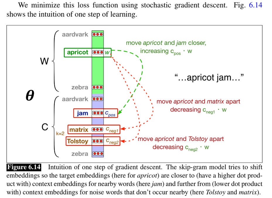
Now that we have the data and an overarching idea of our objective we can formalize this. The description and figure below Jurafski & Martin (2020) Chapter 6 provide a great explanation and formalization on the aim of the Word2Vec learning algorithm.
display.Image("images/model1.png", width=800, height=800)
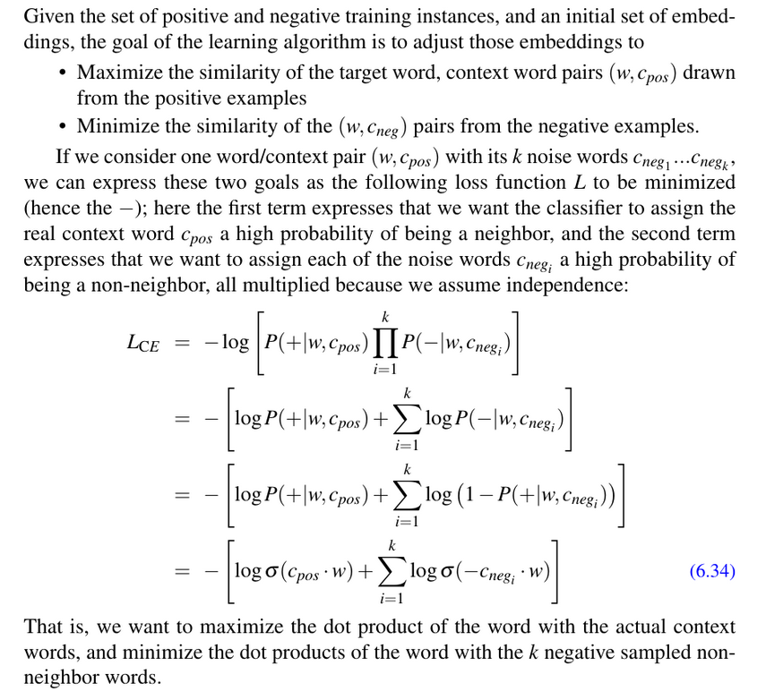
display.Image("images/model2.png", width=800, height=800)
2.1. Parameters and Predictions
def init_params(vocab_size, emb_size, mean, std, seed):
    """ Function to generate random initial parameter matrices

    Args:
        vocab_size (int)
        emb_size (int)
        mean (float): of  normal distribution
        std (float): of normal distribution
        seed (int): to initialize NumPy generator

    Returns:
        list with two matrices randomly generated with the specified dimensions
    """


    # initialize the generator
    generator = np.random.default_rng(seed)

    W = jnp.array(generator.normal(loc=mean, scale=std, size=(vocab_size, emb_size)))
    C = jnp.array(generator.normal(loc=mean, scale=std, size=(vocab_size, emb_size)))

    return [W, C]
params = init_params(len(vocab), emb_size=100, mean=0, std=1, seed=92)
print(params[0].shape, params[1].shape)
(3573, 100) (3573, 100)
@jit
def predict_probs(params, center_idx, contexts_idx):
    """ Estimate the probability of the context words given a center word

    Args:
        params (list): containing the parameters of the model
        center_idx (int): index of the center word
        contexts_idx (list): containing the indexes of the context words

    Returns:
        jax array with one probability for each context word
    """

    # unpack the wegihts matrices: Word embeddings and Context embeddings
    W, C = params[0], params[1]

    # get the W-embedding of the center word
    W_center = jnp.take(W, center_idx, axis=0)

    # get the C-embedding for the context words
    C_contexts = jnp.take(C, contexts_idx, axis=0)

    # similarity score: dot product of word embedding of center word and
    # context embeddings of context words
    similarities = W_center@C_contexts.T

    # finally, in order to transform this similarity into a probability we use
    # the sigmoid function

    return jax.nn.sigmoid(similarities)
# let's see the estimated probabilities for a random example
i = np.random.randint(0, centers.shape[0])
preds = predict_probs(params, centers[i], contexts[i])
print(preds.shape)
print(preds)
(8,)
[1.6075821e-01 5.4325392e-03 9.9648774e-01 4.3908465e-01 9.9913615e-01
 1.2711428e-04 1.0000000e+00 3.6324473e-13]
We can see that we have 8 different predicted probabilities (one for each word in the context). At the moment these probabilities are completely random because we have initialized the parameters randomly. However, we will train the parameters of the model (the embeddings matrices) in order for these probabilities to increase.
# we can use this same function with the negative samples
i = np.random.randint(0, centers.shape[0])
preds_neg = predict_probs(params, centers[i], neg_samples[i])
print(preds_neg.shape)
print(preds_neg)
(80,)
[9.99829412e-01 9.99999881e-01 4.93378907e-01 4.29530472e-01
 5.34372889e-02 7.00894418e-08 3.37184826e-03 8.16896558e-01
 9.99862671e-01 9.73179638e-01 7.99473696e-07 9.99618769e-01
 9.98239517e-01 4.94454755e-03 8.62049311e-03 9.99999523e-01
 1.31775010e-07 9.99997377e-01 1.23342963e-08 7.33995795e-01
 3.76081305e-10 1.17816024e-04 9.99527216e-01 9.99945521e-01
 9.99896884e-01 1.87211007e-01 1.00000000e+00 1.97406393e-02
 7.60079503e-01 1.00000000e+00 4.77221608e-01 4.82995674e-04
 1.94922308e-07 9.29919422e-01 1.10607594e-04 9.93685424e-01
 9.99308825e-01 2.20631175e-02 1.23811606e-03 5.28999045e-03
 9.89047229e-01 9.99425650e-01 2.22090026e-03 8.57670903e-01
 9.88525212e-01 9.90162492e-01 9.98572469e-01 2.50681012e-04
 3.34494910e-03 6.51660741e-07 3.70486727e-04 9.99999762e-01
 9.99999523e-01 9.46112692e-01 9.99999523e-01 9.76181090e-01
 8.53852153e-01 5.88476087e-06 9.99864340e-01 1.19523995e-03
 6.89526722e-02 9.98075247e-01 8.34873378e-01 9.99999046e-01
 9.99998212e-01 7.56851805e-05 9.35527742e-01 9.97949541e-01
 1.14421411e-07 9.99971032e-01 8.74791741e-01 8.16680729e-01
 7.69298669e-09 9.90514040e-01 9.29991841e-01 9.99956012e-01
 7.23925245e-04 6.89373091e-02 2.39428409e-05 1.00000000e+00]
Now we see that we generated 80 probabilities (10 probabilities for each one of the 8 real context words). After training the parameters we want these probabilities to be low!
2.2. Loss function
@jit
def loss_per_example(params, center_idx, contexts_idx, ns_idx, noise=0.000001):
    """ calculate the loss for a center word and it's positive and
        negative examples

    Args:
        params (list): containing the parameters of the model
        center_idx (int): index of the context word
        contexts_idx (list): containing the indexes of the contexts words
        ns_idx (jax array): containing the indexes of the negative samples
        noise (int): small quantity to avoid passing zero to the logarithm

    Returns:
        loss for a single example
    """

    #----------------------------
    # Loss from positive samples
    #----------------------------

    # get the scores for the real context
    preds_pos = predict_probs(params, center_idx, contexts_idx)

    # loss for the positive (real) context words
    loss_pos = jnp.sum(jnp.log(preds_pos + noise))

    #----------------------------
    # Loss from negative samples
    #----------------------------

    # get the scores for all the negative samples
    preds_neg = 1 - predict_probs(params, center_idx, ns_idx)

    # loss for the negative samples
    loss_neg = jnp.sum(jnp.log(preds_neg + noise))

    return -(loss_pos + loss_neg)
# create a vectorized version of the loss using the vmap function from JAX
# the option "in_axes" indicates over which parameters to iterate
batched_loss = jit(vmap(loss_per_example, in_axes=(None, 0, 0, 0, None)))
@jit
def complete_loss(params, all_center_idx, all_contexts_idx, all_ns_idx, noise):
    """ function to calculate the loss for a batch of data by adding the
        individual losses for each example

    Args:
        params (list): containing the parameters of the model
        all_center_idx (list): containing all indexes of center words
        all_contexts_idx (list): containing the indexes for the context words
        all_ns_idx (list): containing all negative samples

    Returns:
        average loss for all examples (float)
    """

    # get all losses from the examples
    losses = batched_loss(params, all_center_idx, all_contexts_idx, all_ns_idx, noise)

    return jnp.sum(losses)/all_center_idx.shape[0]
# use JAX to create a vesion of the loss function that can handle gradients
# the option "argnums" indicates where the parameters of the model are.
# finally use JIT to speed up computations... All JAX magic in one place

grad_loss = jit(value_and_grad(complete_loss, argnums=0))
@jit
def update(params, step, all_center_idx, all_contexts_idx, all_ns_idx, noise, opt_state):
    """ compute the gradient for a batch of data and update parameters
    """

    # calculate the gradients and the value of the loss function
    loss_value, grads = grad_loss(params, all_center_idx, all_contexts_idx, all_ns_idx, noise)

    # update the parameters with a gradient descent algorithm
    opt_state = opt_update(step, grads, opt_state)

    return loss_value, get_params(opt_state), opt_state
2.3. Training
# create some lists to log data
loss_epoch = []

# define vocabulary and embedding size
vocab_size = len(vocab)
emb_size = 100

# training parameters
noise = 1e-8
step_size = 0.001
num_epochs = 20
batch_size = 32

# randomly initialize the two weights matrices
params_seed = 92
params_mean = 0
params_std = 1

params = init_params(vocab_size, emb_size, params_mean, params_std, params_seed)
opt_init, opt_update, get_params = optimizers.adam(step_size)
opt_state = opt_init(params)

# keep track of how many times we are updating the parameters
num_updates = 0

num_batches = math.floor(centers.shape[0]/batch_size)
print(f"Number of batches to process {num_batches} in {num_epochs} epochs")

# train through the epochs
for epoch in range(num_epochs):

    start_time = time.time()

    # IMPORTANT: SHUFFLE EXAMPLES IN EVERY EPOCH!
    indexes = jnp.array(list(range(0, centers.shape[0])))
    shuffled_idx = jax.random.permutation(Key(epoch), indexes)
    centers = jnp.take(centers, shuffled_idx, axis=0)
    contexts = jnp.take(contexts, shuffled_idx, axis=0)
    neg_samples = jnp.take(neg_samples, shuffled_idx, axis=0)

    # split data into batches
    init_index = 0
    end_index = batch_size

    loss_epoch_list = []
    for batch in range(num_batches+1):

        # get the data from the current batch
        batch_idx = jnp.array(range(init_index, end_index))
        batch_centers = jnp.take(centers, batch_idx, axis=0)
        batch_contexts = jnp.take(contexts, batch_idx, axis=0)
        batch_ns = jnp.take(neg_samples, batch_idx, axis=0)

        # calculate gradients and update parameters for each batch
        loss_batch, params, opt_state = update(params, num_updates, batch_centers,
                                                    batch_contexts, batch_ns, noise, opt_state)
        loss_epoch_list.append(loss_batch)
        num_updates += 1

        # update indexes
        init_index = end_index
        # if we are in the last batch...
        if batch == num_batches-1:
            end_index = centers.shape[0]
        else:
            end_index += batch_size

    epoch_time = time.time() - start_time
    loss_epoch.append(sum(loss_epoch_list))

    if epoch%10 == 0:
        print("Epoch {} in {:0.2f} sec".format(epoch, epoch_time))
        print("Loss value: {}".format(sum(loss_epoch_list)))

plt.plot(list(range(num_epochs)), loss_epoch)
plt.show()
Number of batches to process 30052 in 20 epochs
3. Nearest neighbors analysis
Now that we have a numeric representation of all words in the vocabulary, it is possible to calculate distances between these representations.
def build_indexer(vectors, num_trees=10):
    """ we will use a version of approximate nearest neighbors
        (ANNOY: https://github.com/spotify/annoy) to build an indexer
        of the embeddings matrix
    """

    # angular = cosine
    indexer = AnnoyIndex(vectors.shape[1], 'angular')
    for i, vec in enumerate(vectors):
        # add word embedding to indexer
        indexer.add_item(i, vec)

    # build trees for searching
    indexer.build(num_trees)

    return indexer
# create an indexer for our estimated word embeddings (more trees means higher query precision)
indexer = build_indexer(params[0], num_trees=10000)
def find_nn(word, word2idx, idx2word, annoy_indexer, n=5):
    """ function to find the nearest neighbors of a given word
    """
    word_index = word2idx[word]
    nearest_indexes =  annoy_indexer.get_nns_by_item(word_index, n+1)
    nearest_words = [idx2word[i] for i in nearest_indexes[1:]]

    return nearest_words
word = "growth"
N = 20
print(f"{N} nearest neighbors of {word} in the corpus:\n")
print(find_nn(word, word2idx, idx2word, indexer, N))
20 nearest neighbors of growth in the corpus:

['gdp', 'four-quarter', 'slowing', 'slowed', 'productivity', 'annual', 'subdued', 'output', 'slowdown', 'earnings', 'below-trend', 'robust', 'consumption', 'pickup', 'trend', 'real', 'stronger', 'slow', 'momentum', 'contrast']
word = "economy"
N = 20
print(f"{N} nearest neighbors of {word} in the corpus:\n")
print(find_nn(word, word2idx, idx2word, indexer, N))
20 nearest neighbors of economy in the corpus:

['world', 'global', 'capacity', 'potential', 'spare', 'supply', 'activity', 'gradually', 'demand', 'economic', 'whole', 'slack', 'emerging', 'inflationary', 'margin', 'recovery', 'productivity', 'degree', 'expansion', 'rebalancing']
word = "uncertainty"
N = 20
print(f"{N} nearest neighbors of {word} in the corpus:\n")
print(find_nn(word, word2idx, idx2word, indexer, N))
20 nearest neighbors of uncertainty in the corpus:

['considerable', 'about', 'surrounding', 'heightened', 'iraq', 'concerns', 'conflict', 'timing', 'uncertain', 'inherent', 'future', 'risk', 'views', 'regarding', 'magnitude', 'wide', 'relate', 'confidence', 'precise', 'sides']
word = "interest-rate"
N = 20
print(f"{N} nearest neighbors of {word} in the corpus:\n")
print(find_nn(word, word2idx, idx2word, indexer, N))
20 nearest neighbors of interest-rate in the corpus:

['official', 'short-term', 'rates', 'implied', 'path', 'yields', 'long-term', 'repo', 'differentials', 'expectations', 'market', 'forward', 'risk-free', 'basis', 'nominal', 'rate', 'real', 'fomc', 'monetary-policy', 'follows']
word = "inflation"
N = 20
print(f"{N} nearest neighbors of {word} in the corpus:\n")
print(find_nn(word, word2idx, idx2word, indexer, N))
20 nearest neighbors of inflation in the corpus:

['cpi', 'rpix', 'target', 'price', 'expectations', 'rpi', 'medium', 'upside', 'food', 'outturns', 'above-target', 'medium-term', 'near', 'ahead', 'short-term', 'wage', 'beyond', 'drops', 'term', 'twelve-month']
word = "recession"
N = 20
print(f"{N} nearest neighbors of {word} in the corpus:\n")
print(find_nn(word, word2idx, idx2word, indexer, N))
20 nearest neighbors of recession in the corpus:

['crisis', 'downturn', 'much', 'businesses', 'during', 'recessions', 'unemployment', 'start', 'hourly', 'capacity', 'loss', 'full-time', 'beginning', 'mid-', 'period', 'trend', 'participation', 'since', 'companies', 'margin']
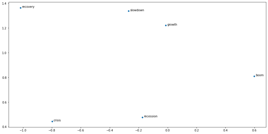
4. Visualization
pca = PCA(n_components=2, random_state=92)
low_dim_emb = pca.fit_transform(params[0])
print(low_dim_emb.shape)
(3573, 2)
words_plot = ["slowdown", "recession", "crisis", "boom",  "growth", "recovery"]
words_idxs = [word2idx[w] for w in words_plot]
low_dim_words = [low_dim_emb[idx] for idx in words_idxs]
low_dim_words = np.array(low_dim_words)
low_dim_words.shape
(6, 2)
df_plot = pd.DataFrame({"x": low_dim_words[:,0], "y": low_dim_words[:,1], "word": words_plot})
df_plot
| x | y | word | |
|---|---|---|---|
| 0 | -0.269677 | 1.337530 | slowdown |
| 1 | -0.173867 | 0.477177 | recession |
| 2 | -0.798840 | 0.444579 | crisis |
| 3 | 0.599359 | 0.810433 | boom |
| 4 | -0.012676 | 1.221398 | growth |
| 5 | -1.017833 | 1.364621 | recovery |
plt.figure(figsize=(16,8))
ax = sns.scatterplot(x=low_dim_words[:,0], y=low_dim_words[:,1])

def label_point(x, y, val, ax):
    a = pd.concat({'x': x, 'y': y, 'val': val}, axis=1)
    for i, point in a.iterrows():
        ax.text(point['x']+.01, point['y'], str(point['val']))

label_point(df_plot["x"], df_plot["y"], df_plot["word"], plt.gca())